Imagine investing thousands in a stunning backyard koi pond or a commercial aquaculture setup, only to battle relentless algae blooms, murky water, and stressed fish due to poor filtration. This common nightmare plagues pond owners and engineers alike, often stemming from overlooked mechanical principles that govern water flow, contaminant removal, and system balance. In this guide, we delve into pond and filter systems through the lens of mechanical engineering, applying core concepts like fluid dynamics, hydraulic design, and pump optimization to achieve crystal-clear water with minimal maintenance and energy use.
As a mechanical engineer with over 15 years of experience in fluid systems design and water treatment, including projects for municipal wastewater ponds and high-density aquaculture facilities, I’ve seen firsthand how treating filtration as an engineered process—rather than a plug-and-play accessory—transforms problematic ponds into thriving ecosystems. Drawing from peer-reviewed studies, EPA guidelines, and real-world applications, this article equips mechanical engineers, pond builders, landscape architects, and advanced hobbyists with actionable insights to design, troubleshoot, and optimize pond and filter setups.
At its core, effective pond filtration addresses key challenges: removing suspended solids (mechanical filtration), converting toxic ammonia to nitrate (biological filtration), and maintaining hydraulic efficiency to prevent dead zones or short-circuiting. Poorly designed systems lead to high biological oxygen demand (BOD), nutrient overloads, and costly interventions like excessive chemical dosing or complete water changes. By integrating principles from fluid mechanics—such as Bernoulli’s equation for pressure drops and Reynolds number for flow regimes—you can minimize head losses, enhance oxygen transfer, and ensure uniform circulation.
We’ll explore fundamentals of pond hydrology, filter types, hydraulic modeling, pump selection, media design, advanced integrations, case studies, maintenance strategies, and emerging sustainable trends. Whether you’re retrofitting a small garden pond or scaling a commercial operation, these engineering-driven approaches will help you achieve superior water quality, reduce operational costs by up to 30% (based on EPA pond optimization data), and promote eco-friendly practices. Let’s engineer clarity—one flow calculation at a time.
1. Fundamentals of Pond Hydrology and Water Quality Challenges
Understanding the hydrological and chemical dynamics of a pond is the foundation for any effective pond and filter system. Ponds, whether natural or man-made, function as closed or semi-closed loops where water quality degrades due to inputs like fish waste, uneaten feed, decaying plants, and atmospheric deposition. Without proper engineering, these factors lead to imbalances that mechanical filtration alone can’t resolve.
1.1 Biological Oxygen Demand (BOD), Ammonia/Nitrite/Nitrate Cycling, and Nutrient Loading in Closed-Loop Systems
Biological oxygen demand (BOD) measures the oxygen consumed by microorganisms as they break down organic matter. In ponds, high BOD from fish excrement or algae die-off depletes dissolved oxygen (DO), stressing aquatic life—fish may gasp at the surface, and anaerobic conditions can release toxic hydrogen sulfide. Engineering solutions involve calculating BOD loading rates: for a stocked koi pond, typical values range from 5-20 mg/L/day, depending on feed input (e.g., 1-2% of fish body weight daily).
The nitrogen cycle is equally critical. Ammonia (NH3) from fish gills and waste is toxic at levels above 0.02 mg/L. Nitrifying bacteria convert it to nitrite (NO2-, still harmful) and then nitrate (NO3-, less toxic but a nutrient for algae). This nitrification process requires oxygen: approximately 4.57 mg O2 per mg NH4-N oxidized. In engineered systems, we design for sufficient residence time and surface area to support these kinetics, often using Monod equations for bacterial growth rates: μ = μ_max * (S / (Ks + S)), where S is substrate concentration, μ_max is maximum growth rate, and Ks is half-saturation constant (typically 1-5 mg/L for ammonia-oxidizing bacteria).
Nutrient loading exacerbates eutrophication. Phosphorus from feed or runoff binds to sediments, releasing during anaerobic events. Engineers must model loading: for a 10,000-gallon pond with 50 kg fish fed 1 kg/day, expect ~10 g N/day input, requiring filtration to maintain total ammonia nitrogen (TAN) below 1 mg/L.
1.2 Common Failure Modes: Algae Blooms, Fish Stress, Sludge Buildup — Root Causes from Poor Hydraulics and Filtration Mismatch
Algae blooms occur when excess nutrients meet sunlight, reducing DO at night via respiration. Root cause: inadequate circulation leading to stratification, where warm surface layers trap nutrients. Fish stress follows from low DO (<5 mg/L) or high TAN, manifesting as lethargy or disease. Sludge buildup in dead zones clogs intakes and harbors pathogens.
These failures often trace to hydraulic mismatches, like undersized pumps causing low turnover (ideal: 1-2 pond volumes/hour) or improper inlet/outlet placement creating short-circuiting. Computational fluid dynamics (CFD) simulations reveal these issues: turbulent flow (Re > 4000) promotes mixing, while laminar flow (Re < 2000) allows settling but risks stagnation.
1.3 Key Water Quality Parameters Engineers Should Monitor (pH, DO, TSS, TAN, ORP)
Monitor pH (7-8.5 optimal for nitrification), DO (>5 mg/L), total suspended solids (TSS <20 mg/L to prevent filter clogging), TAN (<0.5 mg/L), and oxidation-reduction potential (ORP >200 mV for aerobic conditions). Use sensors for real-time data, integrating with PLCs for automated adjustments. Standards from EPA’s pond design manual recommend weekly testing, with thresholds tied to stocking density.
2. Core Types of Pond Filtration and Their Engineering Basis
Pond filtration mimics natural wetlands but is engineered for efficiency. We classify filters by mechanism: mechanical for particulates, biological for dissolved wastes, and adjuncts for specialized treatment. Selection depends on pond volume, loading, and energy constraints.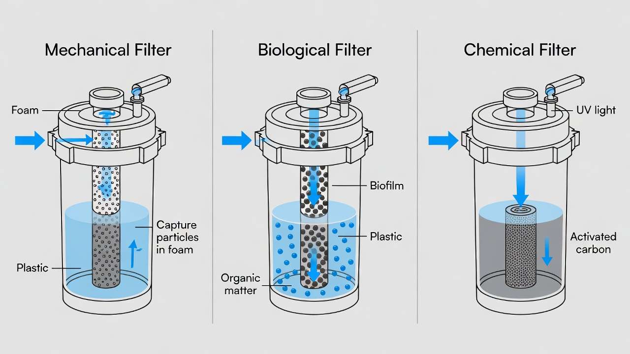
2.1 Mechanical Filtration: Particle Capture Mechanisms (Straining, Sedimentation, Inertial Impaction) — Filter Media Porosity, Flow Velocity Limits, Head Loss Equations
Mechanical filters remove solids via straining (pores smaller than particles), sedimentation (gravity settling in low-velocity zones), and impaction (particles colliding with media due to inertia). Media like foam mats (porosity 0.8-0.9) or sieve screens (100-500 μm) are common.
Flow velocity is key: 0.1-0.5 m/h prevents channeling. Head loss follows Darcy’s law: ΔP = (μ * L * v) / k, where μ is viscosity, L is bed depth, v is velocity, and k is permeability. For a 1 m deep sand bed (k ~10^-4 m^2), expect 0.5-2 m head loss at design flow. Optimize by backwashing when ΔP exceeds 1 m to avoid cake buildup.
2.2 Biological Filtration: Biofilm Kinetics, Nitrification/Denitrification, Surface Area Requirements, Oxygen Transfer Efficiency
Biological filters host biofilms where bacteria perform nitrification. Kinetics follow first-order models at low concentrations: r = k * C, where r is removal rate, k is constant (0.5-2 day^-1 for ammonia), C is concentration.
Surface area (SSA) is crucial: 300-1000 m^2/m^3 for media like K1 plastic. For 1 kg feed/day (producing ~30 g NH4-N), need ~10 m^3 media. Oxygen transfer efficiency (OTE) via aeration or flow: alpha * SOTE, where alpha accounts for wastewater (0.8-0.9), SOTE is standard (20-30% for diffusers).
Denitrification in anoxic zones converts nitrate to N2, requiring carbon sources (e.g., methanol dosing).
2.3 Chemical/UV/Physical Adjuncts: When and Why They Are Used (Coagulation, UV Sterilization, Foam Fractionation)
Chemical adjuncts like alum coagulate phosphates, reducing to <0.03 mg/L. UV sterilizers (254 nm, 30 mJ/cm^2 dose) kill pathogens/algae without residues. Foam fractionation skims proteins via bubbles. Use when biological load exceeds capacity, but engineer for minimal reliance to avoid disrupting microbiomes.
2.4 Integrated vs. Modular Systems: Gravity-Fed vs. Pressurized Designs — Pros/Cons from a Hydraulic Perspective
Integrated systems (e.g., bog filters) use gravity, minimizing energy but risking leaks. Pressurized (e.g., bead filters) allow placement flexibility but increase head (5-10 m). Hydraulically, gravity-fed reduces pump power (by recovering elevation head), ideal for large ponds.
3. Fluid Dynamics and Hydraulic Design Principles for Pond and Filter Systems
Effective pond and filter performance hinges on mastering fluid dynamics. Poor hydraulic design is the single most common reason engineered filtration systems underperform—leading to uneven flow distribution, reduced contact time, excessive energy consumption, and premature media fouling.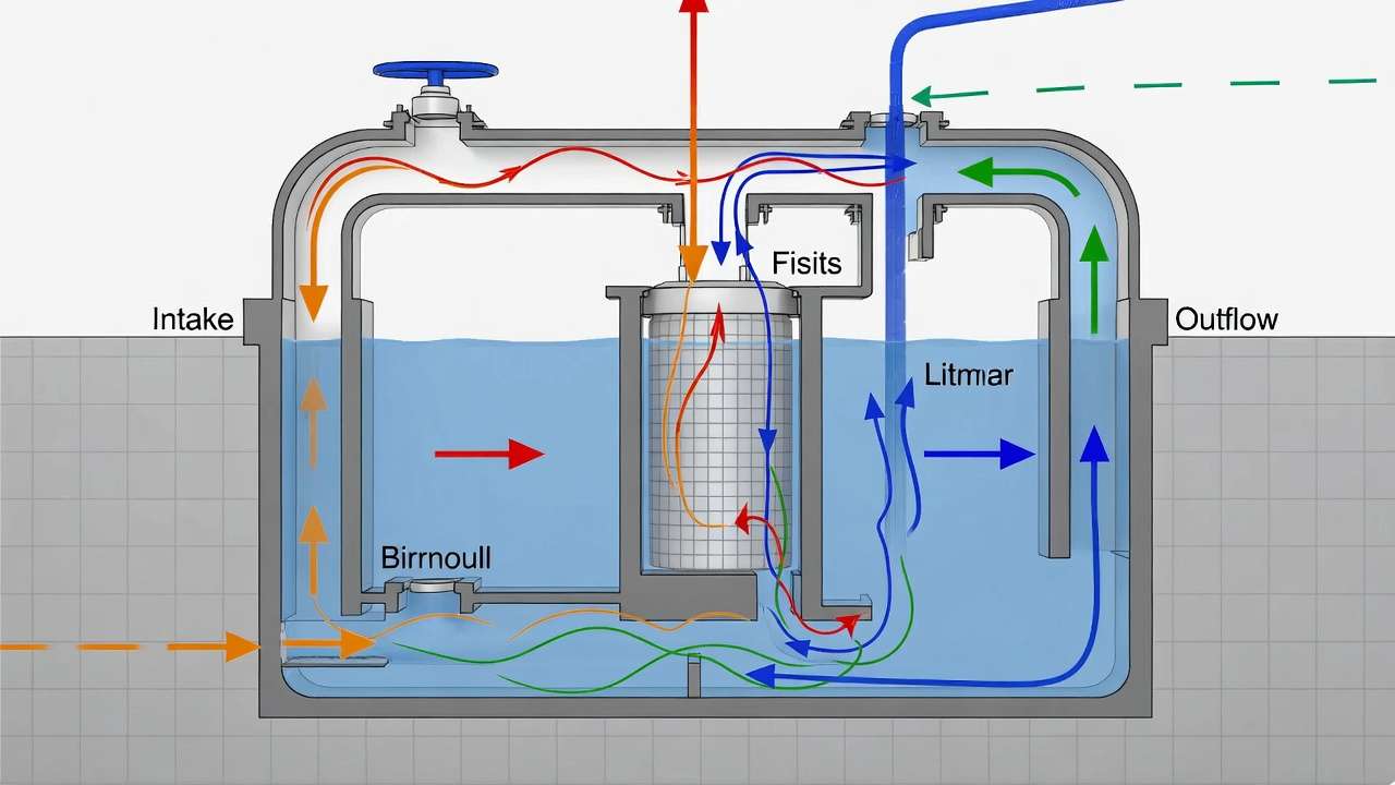
3.1 Bernoulli’s Equation Application to Pond Circulation Loops
Bernoulli’s principle states that along a streamline, the sum of pressure head, velocity head, and elevation head remains constant (neglecting losses): P/ρg + v²/2g + z = constant
In pond loops, this equation helps calculate required pump head. For example, if water is lifted 1.5 m from pond bottom to filter inlet, travels 20 m of 2-inch PVC pipe, and returns via gravity, elevation head is recovered on the return leg—but friction and minor losses must be overcome. Real-world adjustments include adding 10–20% safety margin for filter fouling and fittings.
3.2 Flow Regime (Laminar vs. Turbulent) in Pipes, Filter Chambers, and Media Beds — Reynolds Number Implications
The Reynolds number (Re = ρvd/μ) determines flow behavior:
- Re < 2000 → laminar (smooth, layered flow, poor mixing)
- Re > 4000 → turbulent (chaotic, excellent mixing, higher friction)
In 50 mm pipes at 10 m³/h flow, Re ≈ 70,000 (turbulent), promoting good oxygen transfer but increasing head loss. In media beds, aim for transitional flow (Re 2000–4000) to balance contact efficiency and pressure drop. Laminar flow in oversized chambers creates dead zones; turbulent flow in undersized pipes abrades media or stresses fish.
3.3 Head Loss Calculations: Darcy-Weisbach, Minor Losses (Elbows, Valves, Fittings), Filter Cake Buildup Effects
Major losses use Darcy-Weisbach: h_f = f (L/D) (v²/2g)
where f is the friction factor (from Moody diagram or Colebrook-White equation), L is length, D is diameter, v is velocity. For clean 2-inch PVC, f ≈ 0.02 at Re = 10⁵. Minor losses: K × v²/2g, where K values are 0.9 for 90° elbow, 0.5 for globe valve.
Filter cake buildup dramatically increases resistance—head loss can rise exponentially as porosity drops. Monitor differential pressure across the filter; backwash when Δh exceeds 1.5–2 m (typical threshold for most media).
3.4 Residence Time and Turnover Rate: How to Calculate Ideal Circulation Volume per Hour for Different Pond Volumes and Stocking Densities
Turnover rate is pond volume divided by pump flow rate. Recommended targets:
- Lightly stocked ornamental ponds: 1× per hour
- Moderately stocked koi ponds: 1.5–2× per hour
- High-density aquaculture: 3–5× per hour
Example: For a 20,000 L pond with 100 kg koi (1% feed rate = 1 kg/day), target 2× turnover → 40 m³/h pump. Residence time τ = V/Q should exceed 0.5–1 hour for adequate biological contact in most systems.
3.5 Short-Circuiting, Dead Zones, and Mixing — CFD-Inspired Design Tips Without Full Simulation
Short-circuiting occurs when water takes the path of least resistance, bypassing filter media. Mitigate by strategic inlet/outlet placement (bottom drain inlets, surface skimmer outlets), baffles in filter chambers, and multiple return jets. Dead zones form in corners or under shelves—use velocity vectors >0.05 m/s throughout the pond volume. Simple rule: ensure no path is shorter than 70% of the longest path. For larger ponds, multiple circulation loops prevent stratification.
4. Pump Selection and Energy Optimization in Pond Circulation
Pumps are the heart of any pond and filter system. Incorrect selection wastes energy, causes cavitation, or fails to deliver required flow against system head.
4.1 Pump Curves, System Curves, and Operating Point Determination
Every centrifugal pump has a performance curve showing flow vs. head at a given RPM. The system curve plots required head vs. flow (quadratic due to friction). Intersection is the operating point. Always select a pump where the operating point falls on the efficient portion of the curve (typically 60–80% of BEP—best efficiency point).
4.2 Centrifugal vs. Positive Displacement Pumps — Efficiency at Low vs. High Head
Centrifugal pumps excel at moderate-to-high flow/low-to-medium head (common in ponds). Positive displacement (e.g., lobe, diaphragm) maintain flow regardless of head but are less efficient and noisier—rarely used except in very high-head applications.
4.3 Submersible vs. External Pumps: Cavitation Risk, NPSH, Priming Considerations
Submersible pumps eliminate priming issues and are quieter but harder to service and more prone to overheating if run dry. External (self-priming) pumps allow easy access but require NPSH margin (Net Positive Suction Head) ≥ 1–2 m to prevent cavitation. For deep ponds (>3 m), submersible is often preferred.
4.4 Variable Frequency Drives (VFDs) and Energy Savings in Seasonal/Variable-Load Systems
VFDs adjust motor speed to match demand, following the affinity laws: flow ∝ speed, head ∝ speed², power ∝ speed³. A 20% speed reduction can cut power use by ~50%. Ideal for seasonal ponds (lower flow in winter) or systems with varying fish load.
4.5 Matching Pump Flow to Filter Hydraulic Capacity — Avoiding Under- or Over-Pumping
Over-pumping causes media fluidization (loss of contact time) or excessive backwashing. Under-pumping creates dead zones. Match pump curve to filter manufacturer’s recommended flow range; include a bypass valve for fine-tuning.
5. Filter Media Selection and Bed Design from an Engineering Perspective
Media choice directly impacts removal efficiency, head loss, and maintenance frequency.
5.1 Mechanical Media: Foam, Mats, Brushes, Sieve Screens — Pore Size Distribution, Clean vs. Dirty Head Loss
Foam (30–100 ppi) captures fine particles but clogs quickly. Brushes and Japanese mats offer high surface area with lower head loss. Sieve screens (200–500 μm) provide precise mechanical removal with easy cleaning. Design for staged filtration: coarse → medium → fine.
5.2 Biological Media: K1/K3 Moving Bed, Static Plastic, Lava Rock, Sand — Specific Surface Area (SSA), Void Fraction, Backwashing Frequency
K1/K3 media (SSA 500–900 m²/m³, void fraction ~0.6) excels in moving bed bioreactors (MBBR). Static media (e.g., Bioballs, SSA 200–400 m²/m³) requires less energy but risks channeling. Sand (SSA ~1000 m²/m³ when mature) is effective but heavy and prone to compaction.
5.3 Hybrid and Advanced Media: Bead Filters, Fluidized Beds, Trickling Filters — Pressure Drop Modeling
Bead filters combine mechanical and biological action in pressurized vessels. Fluidized beds offer excellent oxygen transfer but require precise flow control. Model pressure drop using Ergun equation for packed beds: ΔP/L = 150μ(1-ε)²v/(ε³d_p²) + 1.75ρ(1-ε)v²/(ε³d_p)
5.4 Filter Sizing Formulas: Based on Fish Load (kg Feed/Day), TSS Production Rates, Target Turnover
Rule of thumb: 1 m³ media per 1 kg daily feed for lightly stocked systems. For high-density: use 0.5–0.8 m³/kg feed with aeration. TSS production ≈ 25–40% of feed weight; size mechanical filters to handle peak loading.
6. Advanced Design Considerations and System Integration
Beyond basic filtration, professional pond and filter designs incorporate pre-filtration, gravity optimization, piping layout, seasonal adaptations, and automation to achieve long-term reliability and minimal intervention.
6.1 Skimmers, Bottom Drains, and Pre-Filtration Strategies to Protect Main Filters
Effective systems begin with pre-filtration. Surface skimmers remove floating debris (leaves, pollen, uneaten feed) before it reaches the main filter, reducing TSS load by 60–80%. Bottom drains capture settled solids, preventing anaerobic pockets. Install a vortex chamber or settlement sump upstream of mechanical filters to trap heavy particles. This staged approach extends media life and reduces backwashing frequency by 40–70%.
6.2 Gravity-Fed vs. Pressurized Filter Layouts — Elevation Head Recovery, Air Entrainment Prevention
Gravity-fed systems leverage elevation differences: water flows downhill through filters back to the pond, recovering potential energy and minimizing pump power. Pressurized systems allow flexible placement but require higher head (typically 3–8 m). To prevent air entrainment in gravity returns, maintain positive head at the outlet (submerged discharge or waterfall) and slope pipes ≥1% to avoid air locks.
6.3 Tubing/Piping Design: Friction Losses, Velocity Limits (to Prevent Media Abrasion or Fish Injury)
Use Schedule 40 PVC or HDPE for durability. Velocity limits:
- Suction lines: 0.6–1.2 m/s (prevent cavitation)
- Discharge lines: 1.5–2.5 m/s (minimize friction)
- Filter return jets: <0.3 m/s (avoid disturbing fish or substrate)
Calculate total dynamic head (TDH) = static head + friction losses + minor losses + filter head loss. Undersized pipes increase friction exponentially (h_f ∝ v²).
6.4 Winterization, Freeze Protection, and Seasonal Hydraulic Adjustments
In cold climates, lower turnover to 0.5×/hour in winter to conserve energy while maintaining minimum circulation. Use insulated covers, de-icers, or heated lines to prevent freeze damage. Drain external pumps or install heat trace tape. Adjust pump speed via VFD to match reduced biological activity (nitrification slows below 10°C).
6.5 Automation and Monitoring: Flow Sensors, Pressure Differential Switches, DO Probes, PLC/Arduino Integration for Engineers
Modern systems integrate:
- Flow meters (ultrasonic or magnetic) for real-time turnover verification
- Differential pressure transmitters across filters to trigger backwash
- DO, pH, ORP, and temperature probes with 4–20 mA output
- PLC or Arduino-based controllers for automated VFD speed adjustment, pump shutdown on low flow, or alerts via SMS/email
Data logging enables predictive maintenance—e.g., trend head loss to forecast media cleaning.
7. Case Studies and Real-World Engineering Examples
7.1 Small Backyard Koi Pond Retrofit — Before/After Metrics
A 15,000 L koi pond suffered persistent cloudiness (TSS 80 mg/L, TAN 2.5 mg/L) despite a pressurized bead filter. Retrofit: added bottom drain + vortex pre-filter, upgraded to 2× turnover with external centrifugal pump, and installed K1 moving bed (8 m³ media). Results: TSS dropped to <10 mg/L, TAN <0.3 mg/L, energy use reduced 25% (VFD), clarity improved from 30 cm to >1 m visibility within 6 weeks.
7.2 Medium-Scale Water Garden with Bog Filtration — Natural vs. Mechanical Comparison
A 40,000 L water garden used a gravel bog (natural filtration). Issues: uneven flow, plant overgrowth. Hybrid upgrade: added mechanical pre-filter + small pressurized bio-filter for peak loads. Comparison: Bog alone handled base load efficiently (low energy), but hybrid reduced algae spikes by 70% during summer feeding.
7.3 Commercial Aquaculture Pond System — High-Density Design Using Moving Bed Bioreactors (MBBR)
A 500 m³ tilapia system (300 kg/m³ density) used MBBR with K3 media, aeration diffusers, and drum screen pre-filtration. Design flow: 4× turnover. Metrics: Feed conversion ratio improved 15%, ammonia consistently <0.5 mg/L, energy optimized via VFDs tied to DO setpoints.
7.4 Lessons from Failed Installations: Common Hydraulic Mistakes and Fixes
Common errors: undersized returns causing short-circuiting, air-locked gravity lines, mismatched pump/filter curves. Fixes: CFD-informed baffle placement, air release valves, system curve plotting before installation.
8. Maintenance Engineering: Predictive vs. Reactive Approaches
8.1 Backwashing Frequency and Water Loss Minimization Strategies
Backwash when ΔP reaches 1.5–2× clean value or TSS breakthrough occurs. Use timers with pressure override. Minimize water loss via rinse/recycle valves or settling tanks.
8.2 Head Loss Trending as a Diagnostic Tool
Plot ΔP vs. time; exponential rise indicates cake formation or biofilm overgrowth. Sudden jumps signal channeling or media compaction.
8.3 Biofilm Health Indicators and When to Reseed Bacteria
Monitor nitrite accumulation (sign of incomplete nitrification), ORP drop, or ammonia spikes. Reseed with commercial nitrifier cultures after major cleanings or antibiotic use.
8.4 Long-Term Component Lifespan Estimates (Pumps, Media, Liners)
- Centrifugal pumps: 8–15 years with annual seal inspection
- Biological media: 10–20+ years (K1/K3 nearly permanent)
- EPDM liners: 20–30 years with UV protection
9. Sustainability and Future Trends in Pond Filtration Engineering
9.1 Low-Energy Designs and Solar-Assisted Circulation
Solar DC pumps paired with battery storage reduce grid dependency. Floating solar panels double as pond shading to limit algae.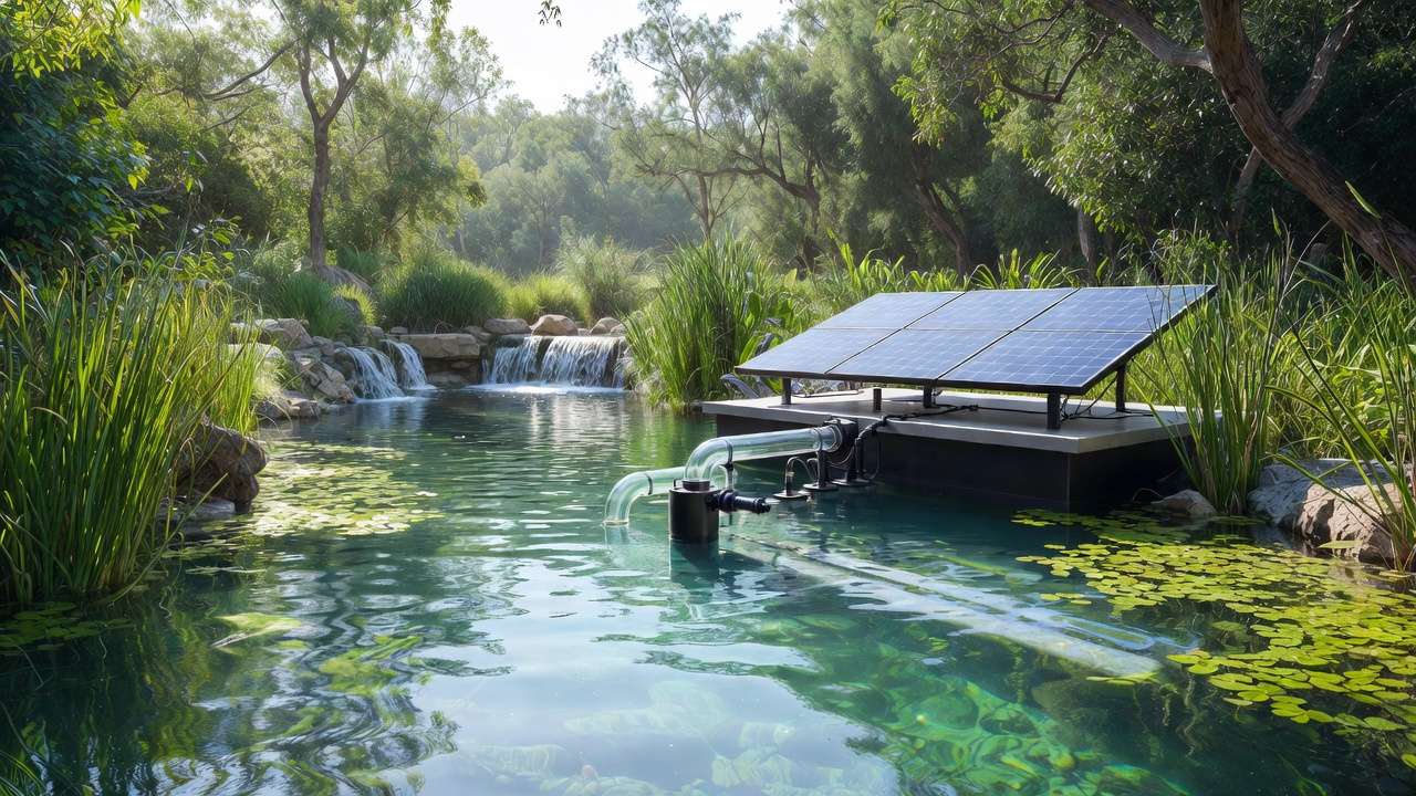
9.2 Nutrient Recovery and Zero-Discharge Concepts
Harvest nitrate-rich backwash water for hydroponics or aquaponics. Implement denitrification reactors with external carbon to achieve near-zero discharge.
9.3 Emerging Technologies: Membrane Bioreactors (MBR), Electrochemical Oxidation, AI-Optimized Flow Control
MBRs provide ultra-fine filtration (<0.1 μm) but require higher energy. Electrochemical systems oxidize organics without chemicals. AI controllers use machine learning on sensor data to dynamically adjust flow, aeration, and backwash—early pilots show 20–40% energy savings.
10. Frequently Asked Questions (FAQs)
Q: How do I calculate required pump head for a 10 ft elevation and 50 ft pipe run? A: Static head = 10 ft. Friction loss (2-inch PVC, 20 gpm) ≈ 4–6 ft (use Hazen-Williams or Darcy). Add 20% safety + filter head (5–10 ft) → total ~20–30 ft TDH.
Q: What SSA is needed for 1 kg daily feed load? A: Conservatively 400–600 m² total protected surface area (e.g., 0.8–1.2 m³ of K1 media at 500–900 m²/m³).
Q: Can I convert a swimming pool pump for pond use? A: Possible, but pool pumps are high-head/low-flow; pond needs moderate-head/high-flow. Check NPSH and seal compatibility.
Q: How often should I backwash a pressurized bead filter? A: Every 3–14 days depending on load; use pressure gauge trigger (typically 8–12 psi rise).
Q: Is a bog filter sufficient alone for a 20,000 L koi pond? A: For light stocking yes; add mechanical pre-filter for heavy feeding to prevent clogging.
Conclusion
Treating pond and filter systems as fully engineered fluid process units—rather than off-the-shelf consumer products—fundamentally changes outcomes. By applying mechanical engineering principles such as hydraulic modeling, precise pump matching, staged filtration, and data-driven maintenance, you can achieve stable, high-quality water with significantly lower energy consumption, reduced chemical dependency, and extended equipment life.
The key takeaway: measure, model, and iterate. Start by auditing your current setup—calculate actual turnover, plot system curves, and monitor key parameters. Small adjustments often yield outsized improvements. Whether you’re designing your first backyard system or optimizing a commercial aquaculture operation, these science-based approaches deliver results that generic guides rarely achieve.
If you’re ready to apply these concepts, sketch your pond layout, note your stocking density and feed rate, and run the calculations outlined here. Share your system specs or questions in the comments—I’d be happy to provide targeted feedback or point you toward additional resources. Engineered clarity isn’t magic; it’s methodical design.